|
Every optimization report answers the question "which parameter values did best?" It cannot answer the more important question: is that ranking real, or did the optimizer just memorize noise? A parameter grid always has a best cell, even on a random walk. If the ranking is noise, the "best" settings carry no information about the future, and trading them means trading a random draw with extra confidence.
Overfitting Analysis measures this directly. After an optimization completes, it replays the question "which parameter combination would I have picked, and how did that pick actually do?" across hundreds to thousands of in-sample / out-of-sample partitions of the same test period, and reports how often the in-sample winner held up. The method is Combinatorially Symmetric Cross-Validation (CSCV) and the Probability of Backtest Overfitting (PBO), from Bailey, Borwein, López de Prado and Zhu (see References below).
Unlike a walk-forward test, which produces one out-of-sample path and keeps only the winner of each window, Overfitting Analysis evaluates every parameter combination on both sides of every split, so it judges the whole family of combinations rather than one survivor, and it produces a distribution of outcomes rather than a single verdict. It also requires no extra data and no additional test runs: the analysis is computed from the daily results of the optimization you already ran, adding at most a few seconds.
The analysis window has two views, chosen with the tabs at its top (or by pressing F again while it is showing): Selection (CSCV / PBO), described first below, asks whether picking the in-sample winner works; Surface (Walk-Forward Correlation) asks a complementary question of the same data -- whether the whole parameter surface, good cells and bad, carries from in-sample to out-of-sample (see Surface View: Walk-Forward Correlation below).
How It Works
1.During the optimization, RealTest records each test’s daily marked-to-market return (the day-over-day change of S.Equity for the combined account).
2.The timeline is cut into S equal blocks (the Blocks setting, default 16). A few trailing days may be dropped to make the blocks equal.
3.Every way of choosing S/2 blocks as in-sample (IS) is enumerated; the other S/2 blocks are out-of-sample (OOS). With 16 blocks that is 12,870 distinct splits.
4.For each split, the parameter combination with the best in-sample Sharpe ratio is selected -- the combination the optimizer would have picked if it had only seen that IS data -- and its out-of-sample Sharpe is ranked against all the other combinations on the same OOS data.
5.The per-split outcomes are aggregated into the headline numbers described below.
Sharpe here is the mean divided by the standard deviation of daily returns (annualized for display). It is used for both selection and ranking regardless of the optimizer’s Score column -- see Limitations below.
Running It
Interactively: check Overfitting Analysis in the Output group of the Optimize dialog and set Blocks if you want something other than 16, then run the optimization as usual. When it completes, a graph window opens showing the analysis.
In a script (which also controls batch runs):
OptimizeSettings:
   OptOverfit: True
   OptOverfitBlocks: 16   // optional; even, 4 to 20
In command line batch mode (realtest -optimize script.rts), the analysis also writes overfit.csv to the OutputPath folder: a summary block (score, haircut, loss chance, fit line, dimensions, warnings) followed by one row per split with its IS and OOS Sharpe, then the Walk-Forward Correlation table (one row per split point) and every combination’s IS and OOS Sharpe at the midpoint split. Remember that batch optimizations only run parameters marked {x}.
The analysis works with Combinatorial, Random, Genetic and Sequential searches (with a caution for the last two -- see Limitations). It cannot be combined with Walk-Forward, Date Intervals, For Each Strategy / Symbol, Shard Processes, or Continue From File, because those runs do not produce one full-period test per parameter combination; the Optimize dialog will say so.
Reading the Results
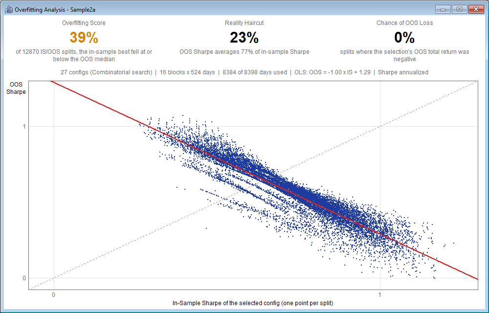
Overfitting Score -- the headline: the percentage of splits in which the in-sample best combination landed at or below the median of all combinations out-of-sample (this is the PBO of the literature). Read it as: how often did picking the in-sample winner work out no better than picking at random?
•50% means coin flip: in-sample rank told you nothing about out-of-sample rank. Optimizing this strategy family is curve-fitting.
•Low values (roughly 25% and below) mean in-sample winners tended to stay winners -- evidence of real, optimizable structure.
•High values (above 50%) mean in-sample winners systematically disappointed -- the classic overfitting signature.
The score is colored green / amber / red at 25% and 45% boundaries. Treat these as orientation, not gospel: the splits reuse the same data and are strongly correlated, so a single optimization’s score has limited resolution -- read 43% vs 48% as "about coin flip" rather than as meaningfully different. More combinations sharpen the ranking; very small grids (under 10 combinations) produce a warning because ranks are then coarse.
Reality Haircut -- across all splits, how much of the in-sample Sharpe evaporated out-of-sample: a haircut of 30% means the OOS Sharpe of the selected combinations averaged 70% of their IS Sharpe. Even genuinely robust strategy families show some haircut (selection always captures some luck); values near 100%, or negative OOS altogether, mean in-sample performance was mostly illusion.
Chance of OOS Loss -- the percentage of splits in which the selected combination’s out-of-sample total return was negative. A blunt, easily-explained floor: how often would the picked settings have actually lost money?
The scatter -- one point per split: x = in-sample Sharpe of the selected combination, y = its out-of-sample Sharpe, with the y = x diagonal and a fit line for reference. The useful reads are where the cloud sits (is OOS performance broadly positive and near the diagonal, or collapsed toward zero?) and how tightly it hugs the diagonal.
Do not expect a positive fit-line slope, and do not read a negative slope as proof of overfitting. Because the x-axis is always the maximum IS Sharpe, splits where the winner won by more luck sit further right and give more of that luck back out-of-sample -- plain regression to the mean. The slope is therefore negative even for genuinely robust strategy families (and even for pure noise). It is shown for completeness; the Overfitting Score and the Reality Haircut are the discriminating numbers.
As a calibration example: a 60-combination moving-average-cross grid on 33 years of SPY, run with 12 blocks (924 splits), produced Overfitting Score 17%, Reality Haircut 17% and Chance of OOS Loss 1%. Reading: the family has genuine common structure (long exposure to an uptrending index), in-sample ranking carried real information about out-of-sample ranking, and almost no split lost money out-of-sample. The scatter’s fit line was nonetheless steeply negative -- the regression-to-the-mean effect described above, not a defect.
Surface View: Walk-Forward Correlation
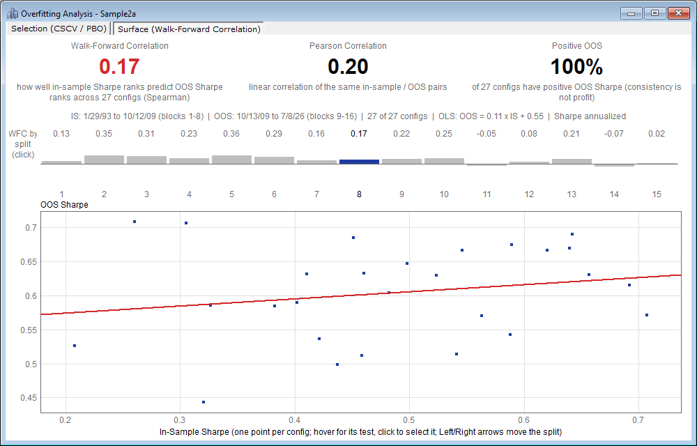
The Overfitting Score judges one decision -- picking the in-sample winner. The Surface view judges the whole parameter surface instead, using the Walk-Forward Correlation (WFC) diagnostic of Martyn Tinsley (see References). The same blocks are split once, chronologically: the first k blocks are in-sample and the rest out-of-sample (the midpoint split by default). Every parameter combination’s in-sample Sharpe is paired with its own out-of-sample Sharpe, and the pairs are correlated across all combinations. If combinations that did well in-sample also did well out-of-sample, and poor ones stayed poor, the optimization surface has persistent structure; if the pairs are a shapeless cloud, the surface is noise and any choice made on it is arbitrary.
Walk-Forward Correlation -- the headline: the Spearman rank correlation of in-sample vs out-of-sample Sharpe across all combinations. +1 means the in-sample ranking was reproduced exactly out-of-sample, 0 means it told you nothing, negative means the ranking inverted. It is colored green / amber / red at 0.5 and 0.2 -- orientation only, since the value depends on the grid you tested (see below). Pearson Correlation is the ordinary linear correlation of the same pairs; a large gap between the two usually means a few extreme combinations are steering the linear fit. Positive OOS is the percentage of combinations whose out-of-sample Sharpe was positive -- reported alongside because consistency is not profit: a surface whose losers stay losers correlates perfectly and makes no money.
Read the two together: high correlation with mostly-positive OOS results suggests structural edge; high correlation with negative OOS results is a consistent loser; low correlation means the surface did not persist, and any good OOS result among the combinations is as likely to be chance. And read them against the Overfitting Score: a robust family with a reliable selection rule shows high WFC and a low score; high WFC with a high score means the surface is real but its exact peak wanders (prefer a plateau or an average of neighbors over the single best cell); low WFC with a low score means selection happened to work despite an unstable surface -- investigate before trusting it.
The split profile -- the strip of bars shows the Walk-Forward Correlation at every possible split point (in-sample = blocks 1 to k), so a single split’s number can be seen in context: a surface that persists shows positive bars across most of the strip, while a lone high bar is a coincidence of where the boundary fell. The highlighted bar is the split being shown; click another bar, or press the Left and Right arrow keys, to move the boundary. The header line gives the in-sample and out-of-sample date ranges of the current split and how many combinations it includes (combinations that never traded on one side have no Sharpe there and are left out).
The scatter -- one point per combination: x = its in-sample Sharpe, y = its out-of-sample Sharpe, each axis scaled to its own data, with the fit line. Hovering a point shows its test number, its parameter values and the two Sharpes; clicking it selects that test in the results list, so an outlying combination can be examined directly.
Two cautions. First, the value depends on the combinations you feed it: a grid padded with obviously bad settings (very short lookbacks, absurd thresholds) will correlate well simply because the bad cells are bad in every period -- which is why the grid should contain only settings you would consider trading, and why Positive OOS is shown alongside. Second, one split is one sample; a history with a regime change near the boundary can show a low correlation for a family that is otherwise stable, which is what the split profile is there to reveal. The screenshot above (Sample2a’s 27-combination moving-average grid on 33 years of SPY, 16 blocks) shows a Walk-Forward Correlation of 0.17 at the midpoint with 100% positive OOS and a profile of mostly small positive bars: a family with a common long-equity edge but only weak persistent ranking among its members -- consistent with its Overfitting Score of 37% on the Selection tab, and a reminder that the two views measure different things.
The Display
The analysis appears as a graph type in the Optimization Results Graphs window and behaves like the other types. It opens automatically when the optimization completes, and closing it loses nothing: the most recent analysis is kept until another optimization with Overfitting Analysis replaces it, and can be re-displayed in any optimization graph window with the F key, the ResGraph menu ("Overfitting Analysis"), or the Options dialog.
•Log Summary Text (ResGraph menu) writes the headline numbers, followed by a table of the Walk-Forward Correlation at every split point, to an untitled Log window -- handy for keeping a text record alongside other notes.
•Show Data (ResGraph menu) opens the current view’s points in a list window, from which they can be copied or saved like any other list: the full split table (Split, IS Sharpe, OOS Sharpe) for the Selection view, or every combination’s IS and OOS Sharpe at the split being shown (Config, Test, IS Sharpe, OOS Sharpe) for the Surface view.
•Copy Image to Clipboard (Ctrl+C), Save Image as PNG File, and the Dark Background option work as in the other graph types.
Choosing the Block Count
Blocks (S) must be even, between 4 and 20. The number of splits is the number of ways to choose S/2 blocks from S: 8 blocks gives 70 splits (coarse; fine for a quick look), 12 gives 924 (good for shorter histories), 16 gives 12,870 (the default), and 20 gives 184,756 (finest; the analysis takes a few seconds).
The trade-off: more blocks give more splits (smoother statistics) but shorter blocks, and each block should still contain enough days to make a Sharpe ratio meaningful -- the analysis warns below 20 days per block. As a rule of thumb, keep the default 16 for ten or more years of daily data and drop to 12 or 8 for shorter histories. The block count is shown with the results because the score depends somewhat on it; when comparing strategies, compare at the same block count.
Limitations
•It reuses the same history. Overfitting Analysis detects selection overfitting -- whether ranking combinations in-sample predicted their relative merit out-of-sample within the data you tested on. It is not a substitute for genuinely untouched data, and it cannot detect the overfitting that comes from trying many different strategy ideas until one fits the era you keep testing on.
•Selection is by Sharpe, whatever your Score column. The analysis asks "does picking the in-sample Sharpe winner work?" even if your optimizer scored by NetProfit, MAR, or a custom formula. Path-dependent scores (anything involving drawdown) cannot be computed on the non-contiguous day sets the method requires. In practice a family with no Sharpe-stable ranking will not have a MAR-stable ranking either.
•Genetic and Sequential searches deliberately spend their tests near in-sample winners, so the tested combinations are not a neutral sample and the score can shift. The analysis still runs but flags a warning; Combinatorial and Random runs give the cleanest readings.
•Combinations that never trade have undefined Sharpe; they are never selected and rank below every trading combination. If many combinations in the grid never trade, a warning appears and the score should be read skeptically.
•Returns are the combined account’s daily mark-to-market, the same series as S.Equity -- including CashInOut/FeesInOut flows if the script uses them, and frozen at zero after a combination wipes out its equity (also warned).
•A stopped or failed optimization produces no analysis, and runs whose returns matrix would exceed about 1 GB (roughly, tests x trading days x 4 bytes) skip it with a note in the error log.
Example
Settings:
   DataFile: sample1.rtd
   BarSize: Daily

OptimizeSettings:
   OptimizeMode: Combinatorial
   OptOverfit: True
   OptOverfitBlocks: 12

Parameters:
   MALen: from 10 to 100 step 10   {x}
   ExitLen: from 5 to 30 step 5   {x}

Strategy: MACross
   EntrySetup: C > Avg(C,MALen)
   ExitRule: C < Avg(C,ExitLen)
Run the optimization from the dialog, or headless with realtest -optimize <script> (which also writes overfit.csv).
References
•Bailey, Borwein, López de Prado, Zhu: The Probability of Backtest Overfitting (Journal of Computational Finance, 2017; SSRN 2014).
•López de Prado: Advances in Financial Machine Learning (Wiley, 2018), chapters 11-12.
•Tinsley: Walk Forward Correlation: A Diagnostic for Over-Fitting and Structural Edge in Trading Strategy Optimisation (SSRN 6324079).
RealTest’s implementation follows the papers’ CSCV/PBO construction, with selection and ranking by Sharpe ratio of daily returns. The Walk-Forward Correlation view applies Tinsley’s diagnostic to the same daily-return matrix, with the same Sharpe metric and with the in-sample / out-of-sample boundary placed at the block boundaries; the split profile is the multi-window extension the paper lists as future work.
|

